
Transfer Learning using PyTorch
Today we learn how to perform transfer learning for image classification using PyTorch.
Introduction
What is PyTorch?
PyTorch is an open-source machine learning library based on the Torch library, used for applications such as computer vision and natural language processing, primarily developed by Facebook’s AI Research lab (FAIR).
What is Transfer Learning?
Transfer learning (TL) is a research problem in machine learning (ML) that focuses on storing knowledge gained while solving one problem and applying it to a different but related problem.
For example, the knowledge gained while learning to recognize cars could apply when trying to recognize trucks.
Getting started
We use a Kaggle Notebook for this task since it provides free computation services which should be sufficient for the image classification task.
Import Libraries
We import various libraries along with the submodules required for the image classification.
%matplotlib inline
%reload_ext autoreload
%autoreload 2

# Import required libraries
import numpy as np
import pandas as pd
import time
import math
import tqdm as tqdm
import os
import csv
import torch
import torch.nn.functional as F
import torch.optim as optim
import torchvision.models as models
import matplotlib.pyplot as plt
from PIL import Image
from torch import nn
from torch.utils.data.dataset import Dataset
from torch.utils.data import DataLoader
from torchvision import transforms, datasets
from torch.autograd import Variable

# Check if compute other than CPU is available
device = torch.device('cuda' if torch.cuda.is_available() else 'cpu')
Load Data
Dataset
We use the 102 Category Flower Dataset for our image classification task. This dataset contains images of flowers belonging to 102 different categories.
Set data folders
data_dir = '../input/oxford-flowers-data/flower_data'
train_dir = data_dir + '/train'
valid_dir = data_dir + '/valid'
test_dir = data_dir + '/test'
name_json = data_dir + '/cat_to_name.json'
Here we have three main directories train_dir, valid_dir, and test_dir which contain training, validation, and testing data respectively.
We also have a cat_to_name.json file which contains the mapping of flower category to the name of the flower.
Load test data
The dataset at hand contains training and validation images categorized inside their respective folders, however, the test images are not categorized and are merged in a single directory.
Thus, we need to define functions to load the test data as required by PyTorch during the training of the model.
def pil_loader(path):
    with open(path, 'rb') as f:
        img = Image.open(f)
        return img.convert('RGB')
class TestDataset(torch.utils.data.Dataset):
    def __init__(self, path, transform=None):
        self.path = path
        self.files = []
        for (dirpath, _, filenames) in os.walk(self.path):
            for f in filenames:
                if f.endswith('.jpg'):
                    p = {}
                    p['img_path'] = dirpath + '/' + f
                    self.files.append(p)
        self.transform = transform

    def __len__(self):
        return len(self.files)

    def __getitem__(self, idx):
        img_path = self.files[idx]['img_path']
        img_name = img_path.split('/')[-1]
        image = pil_loader(img_path)
        if self.transform:
            image = self.transform(image)
        return image, 0, img_name
Label mapping
We load the labels JSON file and define a function to get the class/category of a flower by passing in an index.
import json

with open(name_json, 'r') as f:
    cat_to_name = json.load(f)
def get_cat_name(index):
    return cat_to_name[idx_to_class[index]]
Transform
Now even though we might have enough data for training but performing various transforms or operations on the images helps the model learn better and perform efficiently on unseen data.
mean = [0.485, 0.456, 0.406]
std = [0.229, 0.224, 0.225]

normalize = transforms.Normalize(mean=mean, std=std)
data_transforms = transforms.Compose([
                    transforms.Pad(4, padding_mode='reflect'),
                    transforms.RandomRotation(10),
                    transforms.RandomResizedCrop(224),
                    transforms.RandomHorizontalFlip(),
                    transforms.ToTensor(),
                    normalize
                ])
test_transforms = transforms.Compose([
                    #transforms.Pad(4, padding_mode='reflect'),
                    transforms.RandomResizedCrop(224),
                    transforms.ToTensor(),
                    normalize
                ])
Dataloader
Next, we provide the image dataset directories and the respective transforms to the dataloader function which will actually load images as needed.
train_datasets = datasets.ImageFolder(train_dir, data_transforms)
val_datasets = datasets.ImageFolder(valid_dir, test_transforms)
test_datasets = TestDataset(test_dir, test_transforms)
bs = 64

trainloader = torch.utils.data.DataLoader(train_datasets, batch_size=bs, shuffle=True)
validloader = torch.utils.data.DataLoader(val_datasets, batch_size=bs, shuffle=True)
testloader = torch.utils.data.DataLoader(test_datasets, batch_size=1, shuffle=False)
Finally, we create a dictionary to get the class/category of a flower from an index.
idx_to_class = {val:key for key, val in val_datasets.class_to_idx.items()}
Plot images
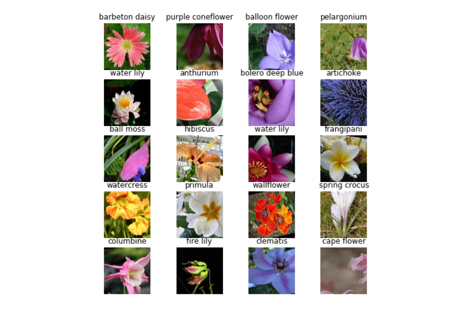
Its always a good idea to take a look at the dataset before training the model. Hence, we define a plot_img function to plot a grid of random dataset images.
def plot_img(preds=None, is_pred=False):
    fig = plt.figure(figsize=(8,8))
    columns = 4
    rows = 5

    for i in range(1, columns*rows +1):
        fig.add_subplot(rows, columns, i)

        if is_pred:
            img_xy = np.random.randint(len(test_datasets));
            img = test_datasets[img_xy][0].numpy()
        else:
            img_xy = np.random.randint(len(train_datasets));
            img = train_datasets[img_xy][0].numpy()

        img = img.transpose((1, 2, 0))
        img = std * img + mean

        if is_pred:
            plt.title(get_cat_name(preds[img_xy]) + "/" + get_cat_name(test_datasets[img_xy][1]))
        else:
            plt.title(str(get_cat_name(train_datasets[img_xy][1])))
        plt.axis('off')
        img = np.clip(img, 0, 1)
        plt.imshow(img, interpolation='nearest')
    plt.show()
plot_img()
Helper functions
Next, we define helper functions which will be required later while training and evaluating the model.
A function that returns accuracy based on the output and target parameters.
def accuracy(output, target, is_test=False):
    global total
    global correct
    batch_size = target.size(0)
    total += batch_size
    _, pred = output.max(dim=1)
    if is_test:
        preds.extend(pred)
    correct += torch.sum(pred == target.data)
    return  (correct.float()/total) * 100
A reset function to reset/clear evaluation metrics.
def reset():
    global total, correct
    global train_loss, test_loss, best_acc
    global trn_losses, trn_accs, val_losses, val_accs
    total, correct = 0, 0
    train_loss, test_loss, best_acc = 0.0, 0.0, 0.0
    trn_losses, trn_accs, val_losses, val_accs = [], [], [], []
A function to record the training and testing stats used to plot graphs.
class AvgStats(object):
    def __init__(self):
        self.reset()

    def reset(self):
        self.losses =[]
        self.precs =[]
        self.its = []

    def append(self, loss, prec, it):
        self.losses.append(loss)
        self.precs.append(prec)
        self.its.append(it)
A function to save checkpoint if a new best score is achieved while training
def save_checkpoint(model, is_best, filename='./checkpoint.pth.tar'):
    if is_best:
        torch.save(model.state_dict(), filename)  # save checkpoint
    else:
        print ("=> Validation Accuracy did not improve")
A function to load a saved checkpoint.
def load_checkpoint(model, filename = './checkpoint.pth.tar'):
    sd = torch.load(filename, map_location=lambda storage, loc: storage)
    names = set(model.state_dict().keys())
    for n in list(sd.keys()):
        if n not in names and n+'_raw' in names:
            if n+'_raw' not in sd: sd[n+'_raw'] = sd[n]
            del sd[n]
    model.load_state_dict(sd)
Cyclic Learning Rate
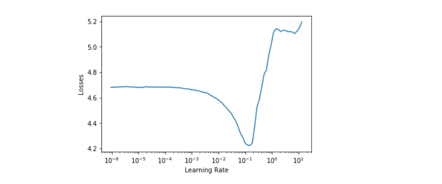
This method is described in the paper Cyclical Learning Rates for Training Neural Networks to find out the optimum learning rate.
The learning rate is increased from a lower value to a higher per iteration for some iterations till loss starts exploding. The learning rate one power lower than the one where loss is minimum is chosen as the optimum learning rate for training.
class CLR(object):
    def __init__(self, optim, bn, base_lr=1e-7, max_lr=100):
        self.base_lr = base_lr
        self.max_lr = max_lr
        self.optim = optim
        self.bn = bn - 1
        ratio = self.max_lr/self.base_lr
        self.mult = ratio ** (1/self.bn)
        self.best_loss = 1e9
        self.iteration = 0
        self.lrs = []
        self.losses = []

    def calc_lr(self, loss):
        self.iteration +=1
        if math.isnan(loss) or loss > 4 * self.best_loss:
            return -1
        if loss < self.best_loss and self.iteration > 1:
            self.best_loss = loss

        mult = self.mult ** self.iteration
        lr = self.base_lr * mult

        self.lrs.append(lr)
        self.losses.append(loss)

        return lr

    def plot(self, start=10, end=-5):
        plt.xlabel("Learning Rate")
        plt.ylabel("Losses")
        plt.plot(self.lrs[start:end], self.losses[start:end])
        plt.xscale('log')


    def plot_lr(self):
        plt.xlabel("Iterations")
        plt.ylabel("Learning Rate")
        plt.plot(self.lrs)
        plt.yscale('log')
Lookahead
Here we implement Lookahead optimizer. As proposed, the Lookahead optimizer goes k steps forward and 1 step backward.
from torch.optim import Optimizer
from collections import defaultdict


class Lookahead(Optimizer):
    def __init__(self, optimizer, alpha=0.5, k=5):
        assert(0.0 <= alpha <= 1.0)
        assert(k >= 1)
        self.optimizer = optimizer
        self.alpha = alpha
        self.k = k
        self.param_groups = self.optimizer.param_groups
        self.state = defaultdict(dict)
        for group in self.param_groups:
            group['k_counter'] = 0
        self.slow_weights = [[param.clone().detach() for param in group['params']] for group in self.param_groups]

    def step(self, closure=None):
        loss = self.optimizer.step(closure)
        for group, slow_Weight in zip(self.param_groups, self.slow_weights):
            group['k_counter'] += 1
            if group['k_counter'] == self.k:
                for param, weight in zip(group['params'], slow_Weight):
                    weight.data.add_(self.alpha, (param.data - weight.data))
                    param.data.copy_(weight.data)
                group['k_counter'] = 0

        return loss

    def state_dict(self):
        fast_dict = self.optimizer.state_dict()
        fast_state = fast_dict['state']
        param_groups = fast_dict['param_groups']
        slow_state = {(id(k) if isinstance(k, torch.Tensor) else k): v
                        for k, v in self.state.items()}
        return {
            'fast_state': fast_state,
            'param_groups': param_groups,
            'slow_state': slow_state
        }

    def load_state_dict(self, state_dict):
        fast_dict = {
            'state': state_dict['fast_state'],
            'param_groups': state_dict['param_groups']
        }
        slow_dict = {
            'state': state_dict['slow_state'],
            'param_groups': state_dict['param_groups']
        }
        super(Lookahead, self).load_state_dict(slow_dict)
        self.optimizer.load_state_dict(fast_dict)
LR Finder
Now, we define the logic to find Learning Rate (LR) using CLR.
def update_lr(optimizer, lr):
    for g in optimizer.param_groups:
        g['lr'] = lr
def lr_find(clr, model, optimizer=None):
    t = tqdm.tqdm(trainloader, leave=False, total=len(trainloader))
    running_loss = 0.
    avg_beta = 0.98
    model.train()
    for i, (input, target) in enumerate(t):
        input, target = input.to(device), target.to(device)
        var_ip, var_tg = Variable(input), Variable(target)
        output = model(var_ip)
        loss = criterion(output, var_tg)

        running_loss = avg_beta * running_loss + (1-avg_beta) *loss.item()
        smoothed_loss = running_loss / (1 - avg_beta**(i+1))
        t.set_postfix(loss=smoothed_loss)

        lr = clr.calc_lr(smoothed_loss)
        if lr == -1 :
            break
        update_lr(optimizer, lr)

        # compute gradient and do SGD step
        optimizer.zero_grad()
        loss.backward()
        optimizer.step()
Train and Test
We implement the train and test logic along with the fit method which will be used in the next step for model training.
def train(epoch=0, model=None, optimizer=None):
    model.train()
    global best_acc
    global trn_accs, trn_losses
    is_improving = True
    counter = 0
    running_loss = 0.
    avg_beta = 0.98
    for i, (input, target) in enumerate(trainloader):
        bt_start = time.time()
        input, target = input.to(device), target.to(device)
        var_ip, var_tg = Variable(input), Variable(target)

        output = model(var_ip)
        loss = criterion(output, var_tg)

        running_loss = avg_beta * running_loss + (1-avg_beta) *loss.item()
        smoothed_loss = running_loss / (1 - avg_beta**(i+1))

        trn_losses.append(smoothed_loss)

        # measure accuracy and record loss
        prec = accuracy(output.data, target)
        trn_accs.append(prec)

        train_stats.append(smoothed_loss, prec, time.time()-bt_start)
        if prec > best_acc :
            best_acc = prec
            save_checkpoint(model, True)

        # compute gradient and do SGD step
        optimizer.zero_grad()
        loss.backward()
        optimizer.step()
def test(model=None):
    with torch.no_grad():
        model.eval()
        global val_accs, val_losses
        running_loss = 0.
        avg_beta = 0.98
        for i, (input, target) in enumerate(validloader):
            bt_start = time.time()
            input, target = input.to(device), target.to(device)
            var_ip, var_tg = Variable(input), Variable(target)
            output = model(var_ip)
            loss = criterion(output, var_tg)

            running_loss = avg_beta * running_loss + (1-avg_beta) *loss.item()
            smoothed_loss = running_loss / (1 - avg_beta**(i+1))

            # measure accuracy and record loss
            prec = accuracy(output.data, target, is_test=True)
            test_stats.append(loss.item(), prec, time.time()-bt_start)

            val_losses.append(smoothed_loss)
            val_accs.append(prec)
def fit(model=None, sched=None, optimizer=None):
    print("Epoch\tTrn_loss\tVal_loss\tTrn_acc\t\tVal_acc")
    for j in range(epoch):
        train(epoch=j, model=model, optimizer=optimizer)
        test(model)
        if sched:
            sched.step(j)
        print("{}\t{:06.8f}\t{:06.8f}\t{:06.8f}\t{:06.8f}"
              .format(j+1, trn_losses[-1], val_losses[-1], trn_accs[-1], val_accs[-1]))
Model and Training
Initialize variables
We initialize all the variables that will be required later while training and evaluating the model.
train_loss = 0.0
test_loss = 0.0
best_acc = 0.0
trn_losses = []
trn_accs = []
val_losses = []
val_accs = []
total = 0
correct = 0
Model
We use a pretrained ResNet50, a variant of the ResNet model which has 48 Convolution layers along with 1 MaxPool and 1 Average Pool layer.
model = models.resnet50(pretrained=True)
Next, we configure the last fully connected layer of the model and save the model checkpoint.
model.fc = nn.Linear(in_features=model.fc.in_features, out_features=102)

for param in model.parameters():
    param.require_grad = False

for param in model.fc.parameters():
    param.require_grad = True

model = model.to(device)
save_checkpoint(model, True, 'before_start_resnet50.pth.tar')
Define loss and optimizer, find learning rate, and plot a graph.
criterion = nn.CrossEntropyLoss()
optim = torch.optim.SGD(model.parameters(), lr=1e-2, momentum=0.9, weight_decay=1e-4)
optimizer = Lookahead(optim)

clr = CLR(optim, len(trainloader))
lr_find(clr, model, optim)
clr.plot()
Training before unfreezing
Let’s load back the ResNet checkpoint that we saved earlier.
load_checkpoint(model, 'before_start_resnet50.pth.tar')
Initialize parameters for the model training.
preds = []
epoch = 30
train_stats = AvgStats()
test_stats = AvgStats()
We reset the parameters to makes sure that we record fresh results while training the model.
reset()
Define loss and optimizer just like before.
criterion = nn.CrossEntropyLoss()
optim = torch.optim.SGD(model.parameters(), lr=1e-2, momentum=0.9, weight_decay=1e-4)
optimizer = Lookahead(optim)
Finally, train the model for 30 epochs.
fit(model=model, optimizer=optimizer)
Save the model checkpoint after training.
save_checkpoint(model, True, 'before_unfreeze_resnet50.pth.tar')
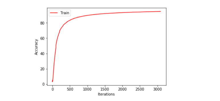
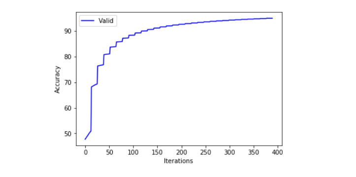
We plot training and validation loss as well as training and validation accuracy graphs to check the model performance.
plt.xlabel("Iterations")
plt.ylabel("Accuracy")
plt.plot(train_stats.precs, 'r', label='Train')
plt.legend()
plt.xlabel("Iterations")
plt.ylabel("Loss")
plt.plot(train_stats.losses, 'r', label='Train')
plt.legend()
plt.xlabel("Iterations")
plt.ylabel("Accuracy")
plt.plot(test_stats.precs, 'b', label='Valid')
plt.legend()
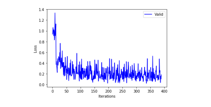
plt.xlabel("Iterations")
plt.ylabel("Loss")
plt.plot(test_stats.losses, 'b', label='Valid')
plt.legend()
Training after unfreezing
Initialize parameters for the model training.
preds = []
train_stats = AvgStats()
test_stats = AvgStats()
We reset the parameters to makes sure that we record fresh results while training the model.
reset()
Enable differentiation tracking for each model parameter.
for param in model.parameters():
    param.require_grad = True
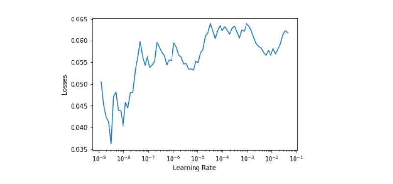
Define the updated loss and optimizer and plot a losses vs learning rate graph.
optim = torch.optim.SGD(model.parameters(), lr=1e-6, momentum=0.9, weight_decay=1e-4)
clr = CLR(optim, len(trainloader), base_lr=1e-9, max_lr=10)
lr_find(clr, model, optim)
clr.plot(start=0)
Let’s load back the resnet checkpoint that we saved earlier.
load_checkpoint(model, 'before_unfreeze_resnet50.pth.tar')
Initialize parameters for the model training.
preds = []
epoch = 10
train_stats = AvgStats()
test_stats = AvgStats()
We reset the parameters to makes sure that we record fresh results while training the model.
reset()
Define the updated learning rate and optimizer for training.
optim = torch.optim.SGD(model.parameters(), lr=1e-9, momentum=0.9, weight_decay=1e-4)
At last, train the model for 10 epochs and save a checkpoint after training.
fit(model=model, optimizer=optimizer)
save_checkpoint(model, True, 'after_unfreeze_resnet50.pth.tar')
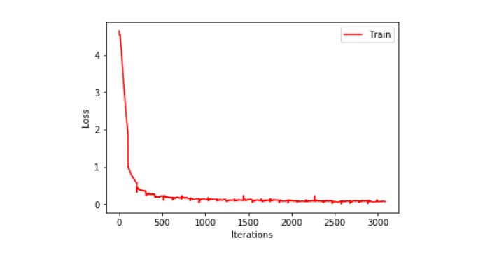
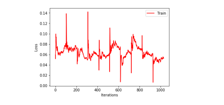
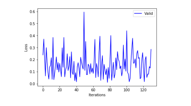
Next, we plot training and validation loss to compare the performance of the model.
plt.xlabel("Iterations")
plt.ylabel("Loss")
plt.plot(train_stats.losses, 'r', label='Train')
plt.legend()
plt.xlabel("Iterations")
plt.ylabel("Loss")
plt.plot(test_stats.losses, 'b', label='Valid')
plt.legend()
Testing
We define a predict method to predict labels for the test dataset.
def predict(img, model):
    model.eval()
    with torch.no_grad():
        input = Variable(img)
        input = input.to(device)
        output = model(input)
        _, pred = output.max(dim=1)
        return pred[0].item()
Predict labels or classes for all the images in the test dataset.
result = dict()
for i, (input, _, path) in enumerate(testloader):
    predicted = predict(input, model)
    result[path[0]] = idx_to_class[predicted]
Save the result for future reference.
csv_file = open('dict.csv', 'w')
writer = csv.writer(csv_file)
writer.writerow(['file_name','id'])
for key, value in result.items():
    writer.writerow([key, value])
csv_file.close()